|
|
|
|
Model behavior...
|
In this section we will get a taste of building mathematical
models. It is a pretty limited taste because all you can do here
is to modify the parameters of the Duffing oscillator. In our
DynaLab
program you will be able to
design your own systems from the beginning. The Duffing
Oscillator Research display is similar to the Duffing Oscillator
display we have been using, but it has additional features to
allow you more control. in the images on this page we depart from
our usual practice of hiding the controls to avoid confusing the
image with the actual applet. What you see here are raw screen shots,
controls included, because the control settings are helpful in
interpreting the images.
Across the top of the display is a row of seven input boxes
and three buttons each under its own label. The input boxes are
where you can change the values of the following
parameters:
1. Forcing Function Amplitude (Ampl)
2. Forcing Function Angular Frequency (Ang Freq)
3. Forcing Function Phase Angle (Phase Ang)
4. Energy Loss Coefficient (Drag)
5. Initial Position (Ini x)
6. Initial Velocity (Ini x')
7. Chronons per cycle (Chr/Cyc)
We have met these parameters before with the exception of the
number of chronons per cycle. Remember that we coined the term
"chronon" to express the notion of the time increment
or "delta t" used in integrating the model differential
equation. Rather than set the size of a chronon directly, we
specify the number of them in a single cycle of the forcing
function. The reason for this is buried in the details of the
integration algorithm.
The three buttons in the top row of controls allow some
manipulation of the high and low limits of the position and
velocity variables. The Open button expands the limits by 25%
with each click. The Close button reduces the limits by the same
amount. The Reset button restores the initial limits. These
limits controls can only be used when the model is not running.
Clicking the Action button disables them. Also because in the
Position/Velocity vs. Time view the limits include the length of
the time axis, we cannot manipulate the horizontal limits in that view. The
remaining row of controls are those we used in previous
displays.
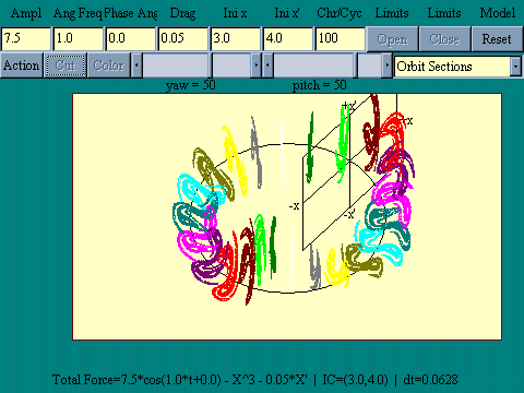
Let's run the research model
beginning with the setup for the chaotic attractor we have been
using. A screen shot from that run is shown at the right.
|
|
|
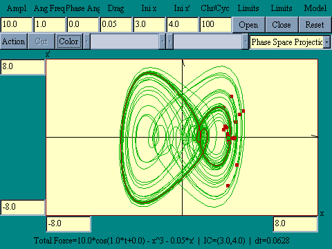
Next let's experiment with some parameter changes. Try
changing the forcing function amplitude to see what effect this
has on the system. Just put in a 10.0 for now. We have done this
for you in the next instance of the
display.
Now here is a trick you should always remember to use when
exploring a new dynamical system. We set the number of chronons
per forcing function cycle at 100 initially so as to not have to
wait too long for some results. The fact that a chronon has a
finite size in model time when in real time it is apparently very
short or perhaps zero, means that the model behavior may be
altered by this artificiality. To check this, after you have
first run a model, increase the chronons per cycle by a factor of
10, in this case to 1000. If you see the same behavior then you
may be reasonable certain that what you are observing comes from
the system itself and not from the model. The
next run
of the model is identical to the
previous one except for that change in the number of chronons per
cycle.
|
|
Now we set the forcing function amplitude back to 7.5 and the
chronons per cycle back to 100 and try something really radical.
Let's make the angular frequency 0.1 and
run the model.
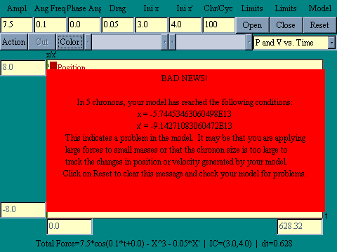
If you ran the model as set up you probably just saw a message
box, which said basically that your model, was out of control. This
box comes up whenever your model variables get to more than a
million times the total span of the viewing window limits. In
this case the viewing limits are set at plus and minus 8 so the
first time the program detects a value of x or x' greater in
absolute value than 1.6e7 the alarm goes off and the message box
comes up. The reported values are those which exceeded the
threshold.
You may clear the message box by clicking on Reset, the model
initial conditions are restored including setting time back to
zero. The 1.6e7 notation by the way represents 1.6 times 10
raised to the 7th power. This is the computer's way of
handling scientific notation.
The purpose of this halting the model is that once a model
becomes unstable, in only a few chronons it can reach extremely
high numbers, beyond the ability of the personal computer to
recognize. If the program is running locally, not off the www,
this does nasty things to the PC including possibly stepping on
some memory in use by the operating system. This would be more
aggravation than the average user would be happy with, requiring
you to re-start your computer with the loss of any data not
written to the disk. By setting the "damage trigger"
relatively low we avoid those interruptions to smooth operation.
If running this as a Java applet, the browser protects the
operating system. In any event, if you are out of bounds by a
factor of a million, chances are your model is bogus in some
way.
Just to get a feel for how rapidly things can get out of hand,
if you did not take notice when the warning message surprised
you take a look at the image here and notice the
reported values on the message box. In absolute value they are roughly
1e14, which is well over 1e6 times the threshold value. That means
that in the last chronon, the model values jumped by at least
that factor.
|
|
|
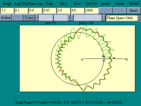
On the bad news box there are a few suggestions as to what
sort of things can cause model instability. One of those is that
the size of a chronon may be too large. When we changed the
angular frequency of the forcing function from 1 to 0.1, we
increased the time to complete a cycle by a factor of 10. Since
the size of a chronon is set by specifying the number of chronons
per cycle, the chronon size was also increased by a factor of 10.
The way to keep an eye on this is to watch the dt = statement in
the bottom margin. In general we need to keep this under about
0.1 time units. Let's go back and fix the model, setting the
angular frequency at 0.1 but increasing the number of chronons
per cycle to 1000. You may see the effect by running
the modified model.
|
|
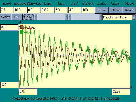
Now let's go the other way with the frequency of the
forcing function. We restore the energy loss coefficient to .05
and put the number of chronons per cycle back to 100. Then make
the angular frequency 10. Run this
new model.
|
|
|
You begin to see some of the power of using mathematical
models. In a few minutes you have learned what it would take
weeks and thousands of dollars to learn in a mechanical lab.
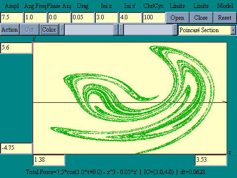
Let's go back to the model and restore the original
parameters of angular frequency = 1, energy loss coefficient of
0.05 and chronons per cycle of 100. Then in the Poincaré Section
view we will see the cross-section of the attractor sliced at
time equal zero with zero phase angle. The
next model
is set up to be centered on the cross-section and zoomed so
that the image nearly fills the drawing area.
|
|
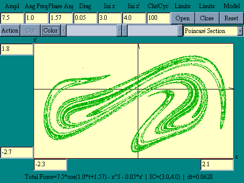
In the
next model
the only change is to introduce a phase angle of pi/2 = 1.57 radians.
Remember that the argument of the cosine in the forcing function is
angular frequency times time, plus the phase angle so any non-zero
phase angle has the effect of shifting the origin of the time axis.
Compare the two Poincaré sections to the two images in the orbit
section view above, one at the (p,v) plane and one 90 degrees from it.
|
|
|
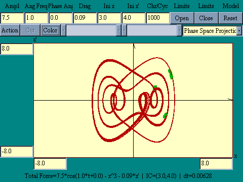
Now if you would, go back to the base
model except we have put in an energy loss coefficient of
0.085 and chronons per cycle of 1000.
If you have followed my suggestions so far, you have seen some
of the techniques by which you can manipulate a mathematical
model to make predictions about the underlying physical reality.
The mathematics of chaos plays a major role in other dynamical
systems also, including growth and decay of ecological systems,
competition for scarce resources and the beating of a human
heart. We will leave the exploration of these ideas for another
course, DynaLab.

For the last time, are there any questions?
|

 Previous
 Other
Other
|
|
|
|


