Splitting hairs...
We have seen previously how as gain changes, the nature of the
attractor changes. We talked about splitting of attractors, known
as bifurcation. We have demonstrated geometrically how this
bifurcation takes place. We have argued that a cascade of
bifurcations is a precursor to chaos. Now we will begin to think
of bifurcations as a characteristic of the logistic function
attractor in phase-control space. We will look at bifurcations as
arising from the mathematical form of iterates of the logistic
function in phase-control space.
In an
earlier section
we wrote expressions for y as a function
of g in developing phase control maps. These functions increased
in complexity exponentially as the iteration number increased but
by actually iterating we were able to produce graphs of these
functions. On the next few displays we will build up a picture by
generating these curves for the first few iterations just to show
how they combine to give an early indication of where these
bifurcations come from. For our case x0=.5, beginning with i2,
even and odd iterations begin to segregate themselves. If you
want to see the images develop you may run through the series of
displays called Bifurcation Beginnings. Otherwise you may just
look at the finished image below each link.
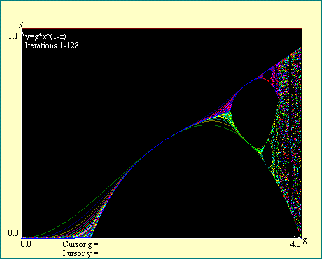 < <
|
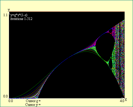
|
As we added higher iterates you should have noticed that the
bundle of odd iterates separates into two groups as does the
bundle of even iterates. This separation of the phase-control
maps of the iterates of the logistic function begins to show
where the bifurcations will occur. As we continue to iterate, the
curves approach the actual point of bifurcation and the break
becomes sharper. In the limiting case of high iteration numbers
the bifurcations become quite distinct. Now we seem to have two
ways, not obviously related, to determine where bifurcation
occurs.
Do bifurcations occur because the slope of the function and
its iterates become steeper than -1 at certain values of gain, or
because the maps of the iterates in phase-control space, where y
is a function of g, wiggle in a certain way? Since both
considerations are equally valid, this must not be an either/or
situation. Perhaps one manifestation of bifurcation derives from
the other or perhaps they both arise from something even more
fundamental. You should not hesitate to use either way of looking
at things as suits your taste, geometry or algebra.
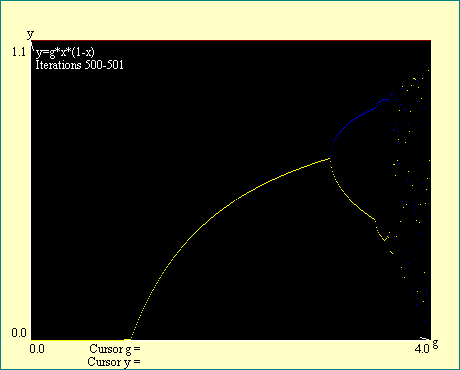
We have previously alluded to the fact that bifurcations
happen faster and faster as you increase gain past 3.0. What we
will try to do next is quantify that phenomena by graphically
locating the points where bifurcations occur. This technique is
not precise but will serve to illustrate a point. To do this we
need to exercise the magnification feature of the program. As we
zoom in on the bifurcations, we will build a table of the gains
at which they occur. You may use the cursor at each display to
verify the tabular value.
In using the cursor to estimate the location of bifurcations
in the logistic function attractor, remember that the precise
location is marked by infinite iteration. Since we iterate only a
finite number of times in the interest of finishing in our
lifetime, you will see the iterates begin to diverge at gains
less than the actual bifurcation. This early divergence then
blends into the real attractor. The best precision will be
obtained by placing the cursor where your eyeball says the blunt
nose of the bifurcation would be if the branches were continued
until they joined.
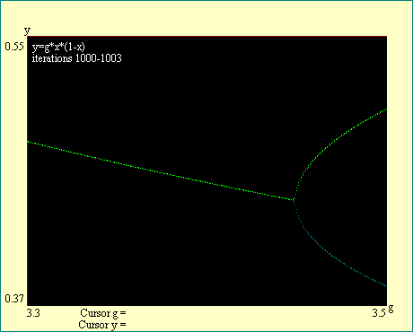
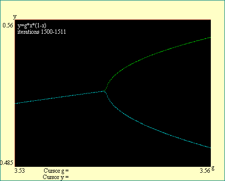
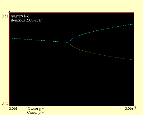
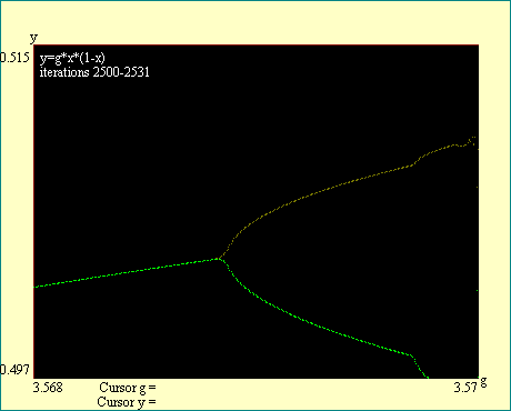
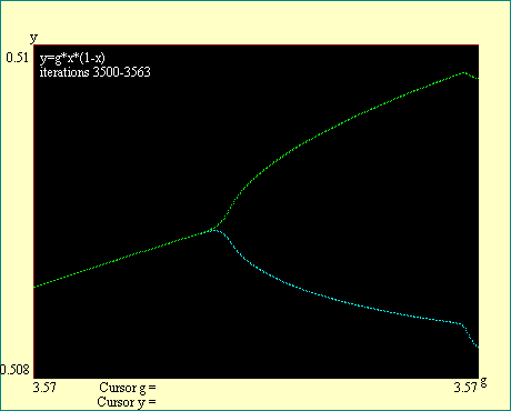
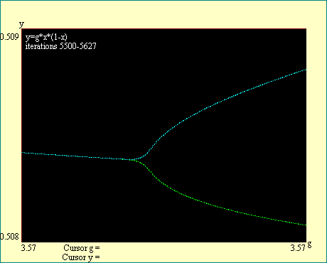
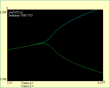
Notice the labels on the display. They tell you in each
instance what the beginning and ending iteration number is. They
also indicate the boundaries of the window to which we have
zoomed. You will see that as we look for the higher order
bifurcations we must iterate more deeply in order to get a
reasonably sharp break at the bifurcation. Also notice that all
branches of the attractor bifurcate at the same gain so that you
may examine any branch to locate the bifurcation. We will locate
the first eight bifurcations in this series of displays. Run the
Cascade Bifurcation series of displays.
|
|
|
|
|
|
|
|
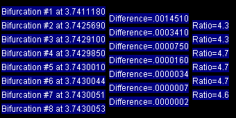
There is a regularity to this cascade of bifurcations we have
been looking at. The rate at which the distance to the next
bifurcation decreases appears to be approximately constant. We
can use the table of bifurcations that we have developed to test
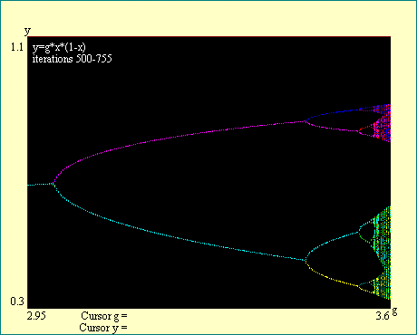
this proposition. On the next display we will see the attractor
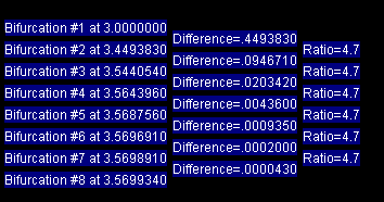
between gain=2.95 and gain=3.6. Immediately below are the 8
bifurcation locations, the 7 differences between adjacent
bifurcations and the 6 ratios of those differences. Even with the
poor precision we are using, the ratios are all close to 4.7. Run
the
Feigenbaum's Number
display.
|
|
When we first explored the map of the logistic function
attractor we found windows of order mixed in with the chaos.
Within these windows there are also cascades of bifurcations. It
is as though at certain values of gain, the attractor collapses
from chaotic behavior to purely periodic, then cascades through
bifurcations back to chaos. It turns out that there are an
infinite number of these windows of order in the regions of chaos
just as there are an infinite number of bifurcations in each
cascade. In each window the attractor has a characteristic
period.
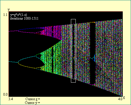
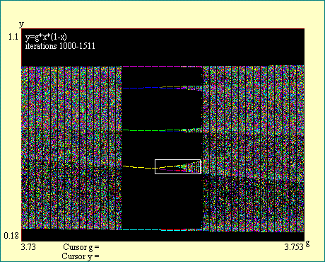
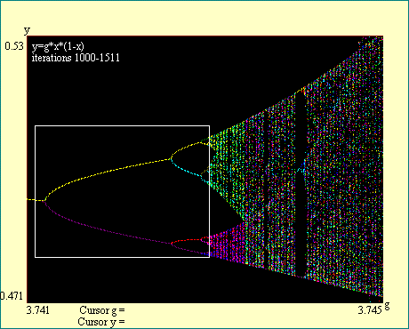
We will examine one of the windows of order in the chaotic
region to illustrate what we have called interior cascades of
bifurcations. First we see the whole map above gain of 3.4 and
then zoom in, magnifying a portion in the region of chaos where
there is one of these windows of order. We have chosen to expand
the picture around a window where the attractor is periodic with
period 5. You will notice the chosen window is outlined in white
as was the case when we first explored the map. Run the Another Window of Order display and its
two zoom displays as well.
|
|
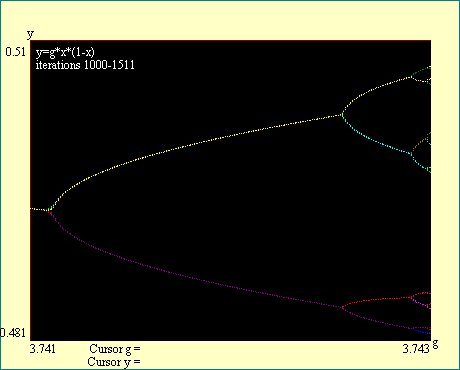
A table of bifurcations, differences and ratios is shown with
the following display. You can see from the table that these
interior bifurcation cascades converge at the same rate as the
original cascade. Exactly why the logistic function attractor
splits with such geometric regularity is not obvious. One would
suppose that the instructions for these bifurcations, as well as
all of the infinitely detailed structure of the two dimensional
logistic function attractor, would be contained in the logistic
function itself. After all, that function contained all the
intelligence we had at the beginning. All we did was iterate it
repeatedly. Run the display
An Interior Feigenbaum Cascade.
|
|
The observation that the logistic function bifurcation
cascades occur with such regularity was first publicized by a
physicist named Mitchell Feigenbaum. The number which the ratios
in our tables approach is approximately 4.6692 and is known as
the Feigenbaum number. Feigenbaum recognized that both the
regularity and infinite variety of the logistic function
attractor have profound implications. Perhaps the instructions
for building complex structures like plants and animals can be
expressed in some relatively simple functions iterated
repeatedly.
In the next lesson we will go on to look at the attractors for
the other functions.

Are there any questions?

 Next
Next
 Previous
 Other
Other


